The Q2R Ising Model and the Arrow of Time
Henry Rachootin
Physicists believe that the universe is time-reversal symmetric, meaning that if one were to reverse the parity and charge of each particle then everything would soundly rewind itself back to the big bang. I’ll call such a system (one for which some simple action would cause it to turn around and rewind) ‘totally reversible.’ Actually doing this to the universe would be physically impossible, but it being totally reversible raises the question: why is it that time always seems to move forward? If the universe that starts now and runs all the way back to the big bang is just as consistent and follows the same rules as the one that starts then and goes until now, then why do we always seem to be moving away from the big bang? The answer comes from thermodynamics: entropy increases over time, and we move forward in the direction of increasing entropy. In much the same way that we have a direction called ‘down’ since we are near a very special patch of space called the Earth with lots of mass, we have a direction called ‘future’ because we are near a very special patch of space-time called the Big Bang with little entropy. However, how can it be that such a reversible process can have such irreversible effects at large scales over long times? At a tiny scales, no one can say if a recording of the real world is playing forwards or backwards, but somehow this time symmetry breaks at large scales.
In [1], Lindgren and Olbrich present a highly simplified model of physics called the Q2R Ising Model automaton which is totally reversible, and prove that it does exhibit a large scale irreversible increase in entropy. It is a one dimensional cellular automaton in which each cell’s state is a spin of either up (1) or down (-1). On each time step every other cell updates its state by flipping its spin if and only if it has one spin up neighbor and one spin down neighbor, so that the even numbered cells and odd numbered cells update on alternate steps. If we say that two adjacent matching spins contribute +1 to the total energy of the system, and two adjacent mismatched spins contribute -1, then these spins flip whenever doing so would not change the total energy. By alternating evens and odds, we ensure that the automaton is totally reversible; if we take a state and translate it left or right by one cell, it will evolve backwards to its initial condition. A sample of the automaton from a random initial condition is shown in Figure 1.
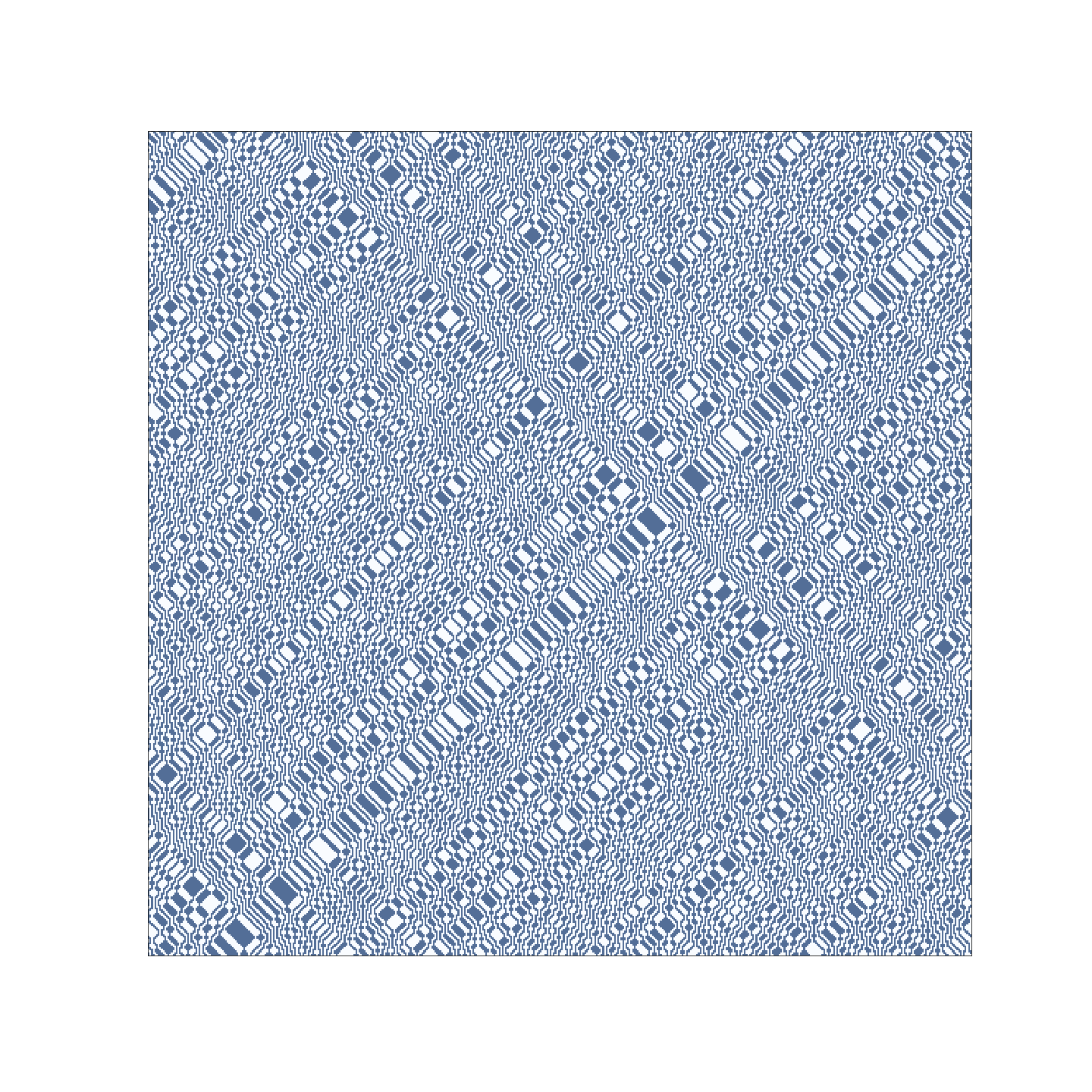
Figure 1: Sample evolution of the Q2R automaton with a random initial condition. Blue cells are up, white cells are down, and time moves from top to bottom (or bottom to top, since it is totally reversible).
Lindgren and Olbrich analyze the system mathematically, and find that if the automaton starts with a random distribution of ups and downs with some bias towards one or the other, it will converge (in the mean) over time to an even distribution of ups and downs. They define the entropy of the system by how far it is from an even distribution, so I use the overall probability of a cell being spin up as a stand-in for entropy. The further the probability gets from 0.5, the lower the entropy. States with high entropy (near p=0.5) are said to be in equilibrium. I use a program to simulate the Q2R automaton, and find that their analysis was correct, as shown in Figure 2, where the probability stays near 0.5 for any initial probability.
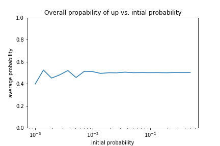
Figure 2: Long term probability of a cell being spin up from different initial probabilities. All initial probabilities converge in the mean to 0.5, showing that the system always approaches equilibrium at large space and time scales.
However, a different story emerges when we look at the actual graphs of the probability over time, as shown in Figure 3.
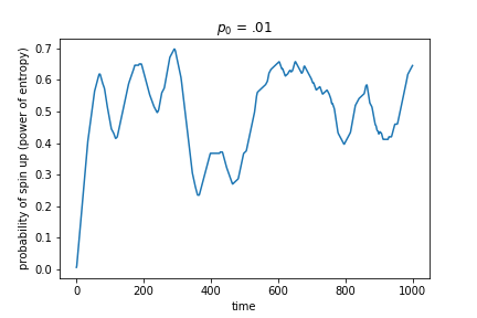
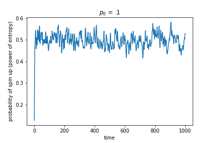
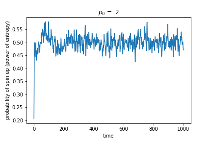
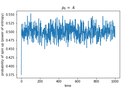
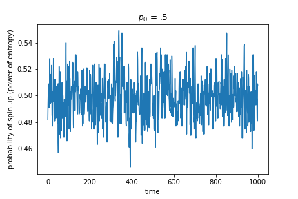
Figure 3: Instantaneous probability that a cell is spin up over time from different initial probabilities. All initial probabilities quickly hover around 0.5, but the variance around that mean depends on the initial entropy.
It looks like the probability varies more over time for initial conditions with low initial entropy (starting strongly biased towards down) while always hovering around 0.5. Indeed, when we graph the variance of the probability for different initial entropy values, we get a power law relationship, as shown in Figure 4.
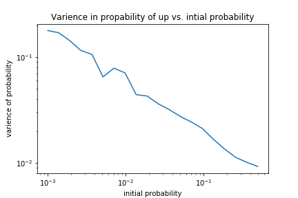
Figure 4: Variance in instantaneous probability that a cell is spin up for different initial conditions. This variance is roughly analogous to the real world concept of temperature, so the fact that it depends on the initial entropy is not a good sign for the explanatory value of this model.
This is not what we would expect from the real world. In reality two systems which start with different entropy will approach the same equilibrium and hover around it with the same variance, if they have the same temperature. In this model it is as if initial entropy and temperature are coupled, and there is no way to uncouple them. This casts some doubt on the explanatory value of the model, since it fails to capture the fact that entropy and temperature are not totally coupled.
While this model demonstrates that a totally reversible system can exhibit large scale irreversible behavior, it cannot offer an explanation that fits within our understanding of thermodynamics in the real world. Perhaps it is the totally determined nature of this simulation that causes this flaw. When the state of the system is completely determined at each time, there can be no concept of instantaneous temperature. As a next step, I would like to make the state of the automaton a probability distribution of all the possible states of the lattice (2^n states) and then evolve that distribution following the Q2R rule. The model includes a measure of total energy, so in a distribution of states that makes the distribution of total energies exponential, the beta parameter of that distribution would be the reciprocal temperature, and that temperature could might then be decoupled from the entropy. In fact, since energy is conserved in the model, temperature would be as well. Unfortunately, the computational memory needed to represent such a distribution and the processor time needed to loop over it would be enormous, so some kind of MCMC numerical method would be needed to simulate that model.
The code for this project can be viewed here or run here.
[1] Lindgren, K. & Olbrich, E. J. The Approach Towards Equilibrium in a Reversible Ising Dynamics Model: An Information-Theoretic Analysis Based on an Exact Solution. Stat Phys (2017) 168: 919. https://doi.org/10.1007/s10955-017-1833-8